The DL_MESO package is supplied with a number of test cases to demonstrate the features of both the Lattice Boltzmann Equation (LBE) and Dissipative Particle Dynamics (DPD) codes. The input files required for these example simulations can be found in the DEMO directory of the package, along with some sample output files. Full details of the test cases can be found in the DL_MESO User Manual.
The following images (full-size versions available by clicking on the thumbnails) and videos are illustrations of the outputs that can be obtained from the test cases, as created using Paraview and VMD. They are freely available to download and use, but please consider citing their source: the DL_MESO website at www.ccp5.ac.uk
If you would like to contribute a new test case for DL_MESO and provide images or videos for this page, please contact Michael Seaton at michael.seaton@stfc.ac.uk
Lattice Boltzmann Equation (LBE)
2D_Pressure
A single fluid is modelled on a 42×42 grid using fixed density boundary conditions on the left and right boundaries to represent a pressure drop across the system, which is bounded by solid walls at the top and bottom. This generates a pressure-driven (Poiseuille) laminar flow with a parabolic velocity profile.
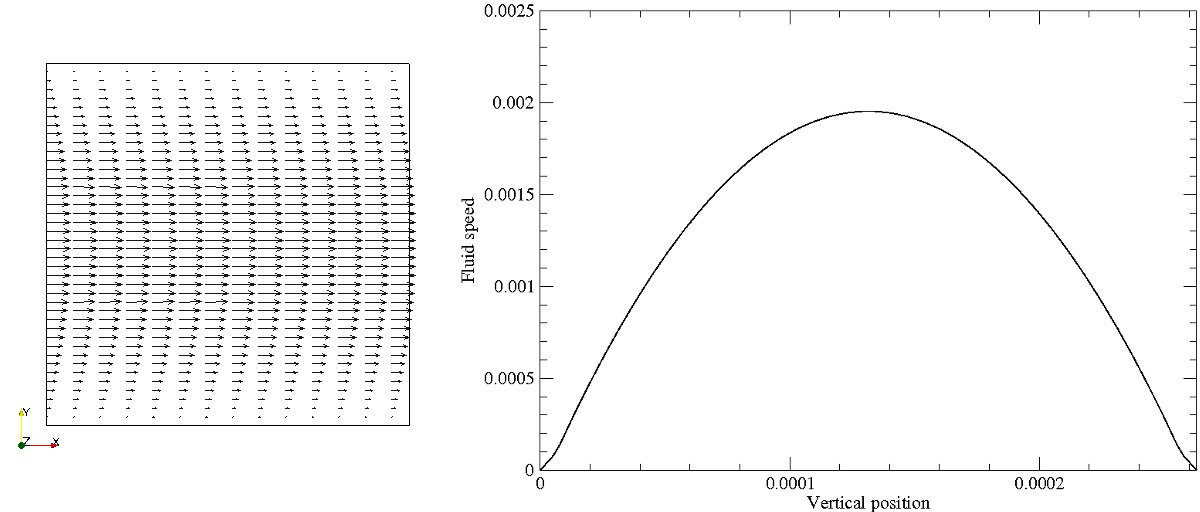
Velocity vector plot (left) and graph of fluid speed against vertical position (right)
2D_Shear
A single fluid is modelled on a 42×42 grid using fixed velocity boundary conditions at the top and bottom boundaries to generate linearly shearing (Couette) flow.
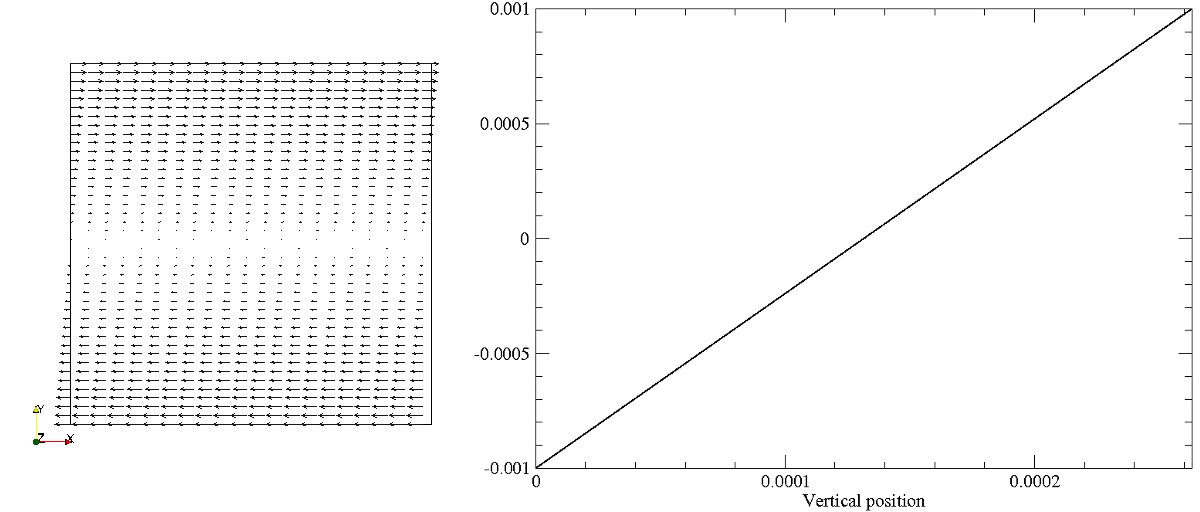
Velocity vector plot (left) and graph of fluid speed against vertical position (right)
2D_CylinderFlow
A single fluid is modelled on a 125×50 grid with solid walls at the top and bottom and a circular obstacle representing an infinitely-long cylinder. A constant body force is applied on the fluid to give a pressure drop across the system and thus cause flow past the cylinder.
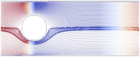
Velocity streamlines coloured by density (scale: blue to red) of flow past a stationary cylinder
2D_KarmanVortex
A single fluid is modelled on a 250×50 grid with a circular obstacle, solid walls at the top and bottom and a constant body force to provide pressure-driven flow. The flow past the cylinder eventually develops into a von Kármán vortex street, involving unsteady vortex shedding at the back of the obstacle. (Video)
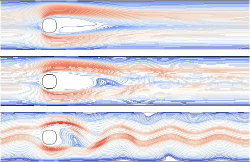
Velocity streamlines coloured by speed (scale: blue to red) before (top), at start of (middle) and during (bottom) vortex shedding
2D_LidCavity
A single incompressible fluid is modelled on a 128×128 grid with a constant velocity boundary condition at the top and solid walls around the other boundaries. The boundary conditions give the equivalent of a container with a sliding lid, resulting in lid-driven cavity flow.

Velocity streamlines coloured by speed
2D_RayleighBenard
An initially stationary fluid on a 102×51 grid is modelled between two solid walls: the wall at the bottom is maintained at a higher temperature than that at the top. With an additional lattice for heat flows, an initial temperature perturbance and buoyancy forces as per the Boussinesq approximation coupling fluid flows and heat transfers [1], the system eventually undergoes natural (Rayleigh-Bénard) heat convection.

Colour map (scale: blue to red) of temperature with superimposed convective velocity streamlines
2D_DropShear
An initially static drop is placed on a 150×50 grid of immiscible continuous fluid close to a solid boundary at the bottom: the system is then sheared using a constant velocity boundary condition at the top. Interfacial forces between the drop and the surrounding fluid are modelled using the Lishchuk continuum-based algorithm [2]. (Video)
Colour maps (scale: blue to red) of fluid density (pressure) and drop shapes/positions over time (top to bottom)
2D_PhaseSeparation
A fluid is modelled on a 50×50 grid with periodic boundary conditions, using Shan-Chen pseudopotentials defined to give a cubic (Peng-Robinson) equation of state [3]. Initially at an intermediate density, the fluid separates out into a liquid drop surrounded by vapour.
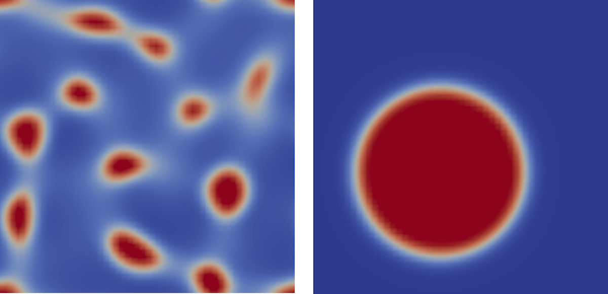
Colour maps of fluid phases (blue: vapour, red: liquid) at early (left) and later (right) stages of separation process
3D_PhaseSeparation
Two immiscible fluids are modelled on a 100×100×100 grid with periodic boundary conditions. Initially mixed together, they are subjected to interfacial forces using the Shan-Chen pseudopotential algorithm and made to separate from each other. (Video 1, Video 2)
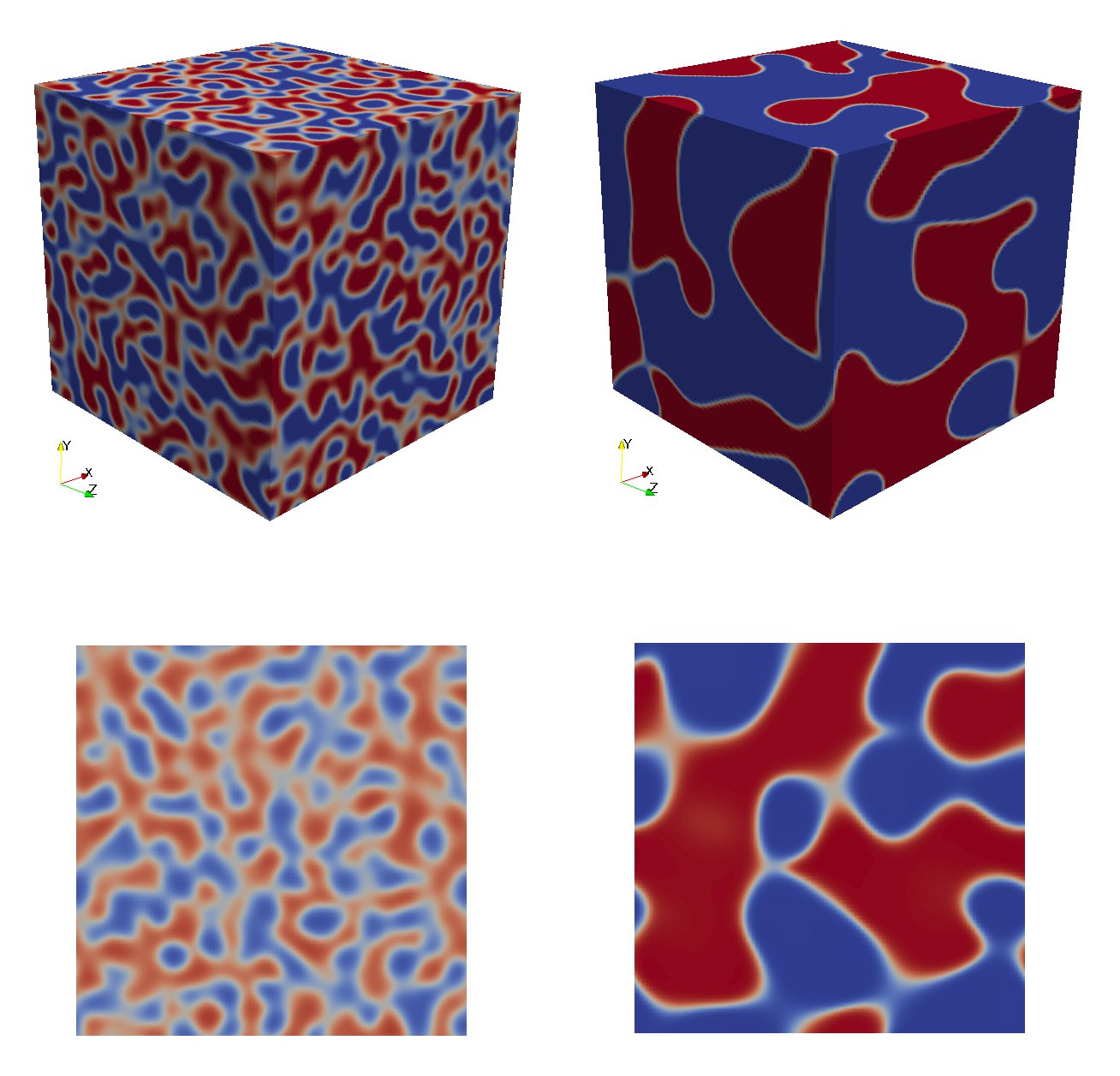
Colour maps of fluid phases (blue and red fluids) at early (left) and later (right) stages of separation process: top images show 3D system, bottom images show 2D slices
3D_Shear
A single fluid is modelled on a 40×30×25 grid with fixed velocity boundaries at the top and bottom. Applying velocities of equal magnitude and opposite direction to those boundaries, a linearly shearing (Couette) flow pattern is produced.
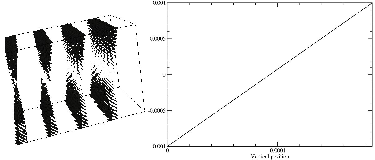
Velocity vector plot (left) and graph of fluid speed against vertical position (right)
3D_RayleighBenard
A stationary fluid on a 80×40×80 grid is modelled between two solid walls at the top and bottom, the latter held at a higher temperature than the former. An additional lattice for heat flows, an initial temperature perturbance and Boussinesq buoyancy forces were applied [1] and the system undergoes natural (Rayleigh-Bénard) heat convection.
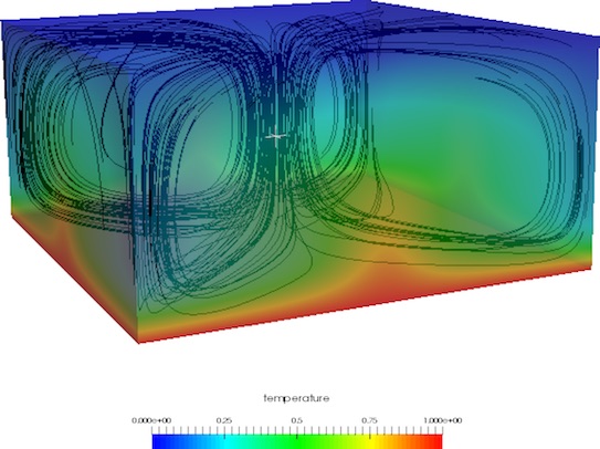
Colour map of temperature with superimposed convective velocity streamlines
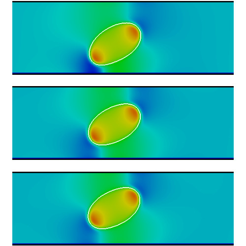
3D_DropShear
An initially static drop is placed on a 150×50×50 grid of immisicible continuous fluid close to a solid boundary at the bottom: the system is then sheared using a constant velocity boundary condition at the top. Interfacial forces between the drop and the surrounding fluid are modelled using the Lishchuk continuum-based algorithm [2].
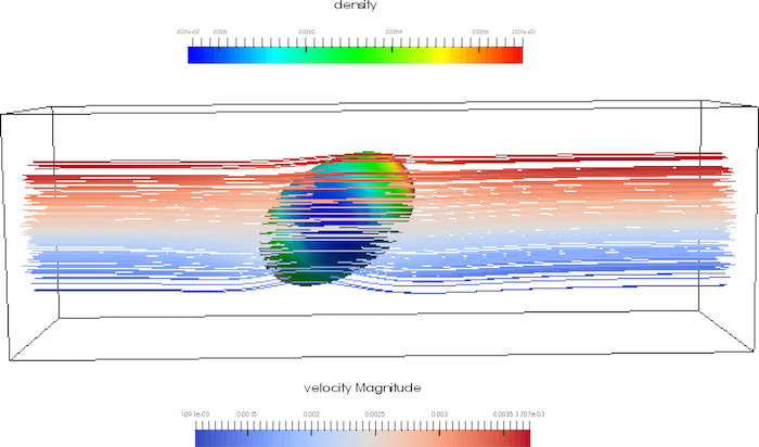
Flow streamlines (coloured by speed) past immiscible drop coloured by fluid density on surface
Dissipative Particle Dynamics (DPD)
Mixture_Small
1000 particles consisting of three species are modelled in a periodic cubic box: their sizes and masses are identical but the repulsive energy parameters are different for each species and default mixing rules are used to determine interactions between particles of different species.
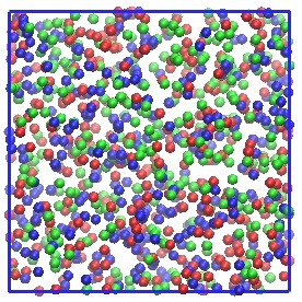
Snapshot of system at final time step (particle species: red, blue and green)
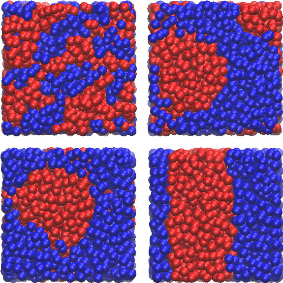
Mixture_Large
256 000 particles consisting of two species of equal sizes and masses but different repulsive parameters are modelled in a periodic cubic box. Standard mixing rules are used to determine the interactions between particles of different species.

Snapshot of system at final time step (particle species: red and blue)
PhaseSeparation
3000 particles of two different species are modelled in a periodic cubic box. The interaction (repulsive) energy parameter between particles of unlike species is significantly higher than those between particles of the same species, causing the two particle species to separate from each other. (Video)
Snapshots of system during separation process from top left to bottom right (particle species: red and blue)
Aggregate
3000 loose particles (making up a solvent) and 30 molecules made up of 10 particles each (with the particles bonded together) are modelled in a periodic cubic box. The repulsive interaction parameter between the solvent and molecule particle species is higher than those between particles of the same species, thus making the molecule hydrophobic and causing them to aggregrate.
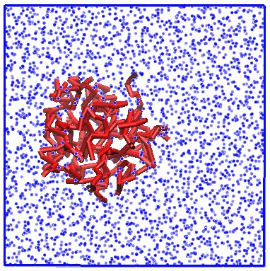
Snapshot of system showing aggregation of hydrophobic molecules (red) in solvent (blue)
Polyelectrolyte
Two simulations are carried out with a slightly hydrophobic polymer of 50 particles immersed in a salt solution consisting of particles for water, positively-charged salt cations and negatively-charged anions. In one case, the polymer is also positively charged to produce a polyelectrolyte and some water particles are substituted with negatively-charged counterions to balance the charges. Charged interactions are calculated using Ewald summation with Slater-like (exponential) charge smearing [4] and a higher radius of gyration is observed for the charged polyelectrolyte compared with the neutral polymer.
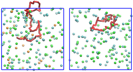
Snapshots of systems with a charged polyelectrolyte (left) and neutral polymer (right), with salt cations (green), anions (cyan) and counterions (orange)
AmphiphileMesophases
Four simulations are carried out of 12 000 particles consisting of amphiphilic dimers (molecules of a hydrophilic particles and a hydrophobic particle bonded together) and a monomer solvent [5]. Different compositions of amphiphilic dimers are used in each of the simulations to produce different mesophases.

Snapshots of systems with isotropic dimer (top left), hexagonal dimer (top right), lamellar dimer (bottom left) and isotropic monomer (bottom right) phases, shown as isosurfaces of hydrophobic particles in dimer molecules
VesicleFormation
37 440 unbonded water particles and 1008 molecules, each consisting of one hydrophobic head particle and three hydrophobic tail particles bonded together, are simulated in a periodic cubic box [6]. The molecules represent amphiphiles and eventually self-assemble into a vesicle, encapsulating a number of water particles inside it. (Video)
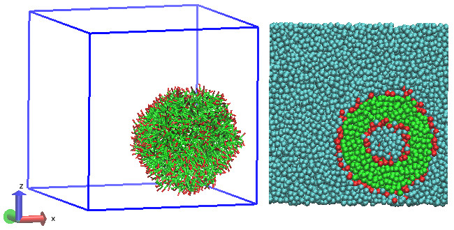
Snapshot of simulation with self-assembled vesicle (hydrophilic heads: red, hydrophobic tails: green) at last time step (left) and cross-section through vesicle (right) illustrating encapsulated water (cyan)
LipidBilayer
35 152 unbonded water particles and 12 000 molecules, each consisting of one hydrophilic head particle and six hydrophobic tail particles bonded together, are simulated in a periodic box [7]. Bond angles are controlled using a potential acting between adjoining pairs of bonds. The molecules represent amphiphilic lipids and eventually self-assemble into a bilayer with the two layers of hydrophobic tails keeping out water.

Snapshot of simulation with self-assembled bilayer (hydrophilic heads: red, hydrophobic tails: green) at last time step surrounded by water (cyan)
PoiseuilleFlow
3000 unbonded particles are simulated in a box with walls of frozen particles added to give no-slip boundaries and a constant body force to give pressure-driven flow. This gives a time-averaged velocity profile that is similar to the parabolic profile expected for laminar Poiseuille flow.
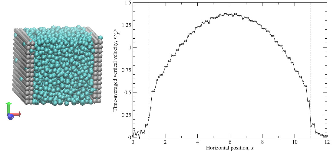
Snapshot of simulation (left) with fluid (cyan) and wall (grey) particles, and time-averaged velocity profile across system (right)
ShearFlow
3000 unbonded particles are simulated in a box with Lees-Edwards shearing boundary conditions and using the Stoyanov-Groot thermostat to apply viscosity and temperature control. A linearly shearing (Couette) flow profile is produced as a result, allowing for the calculation of shear rate and a constant system-wide shear stress.
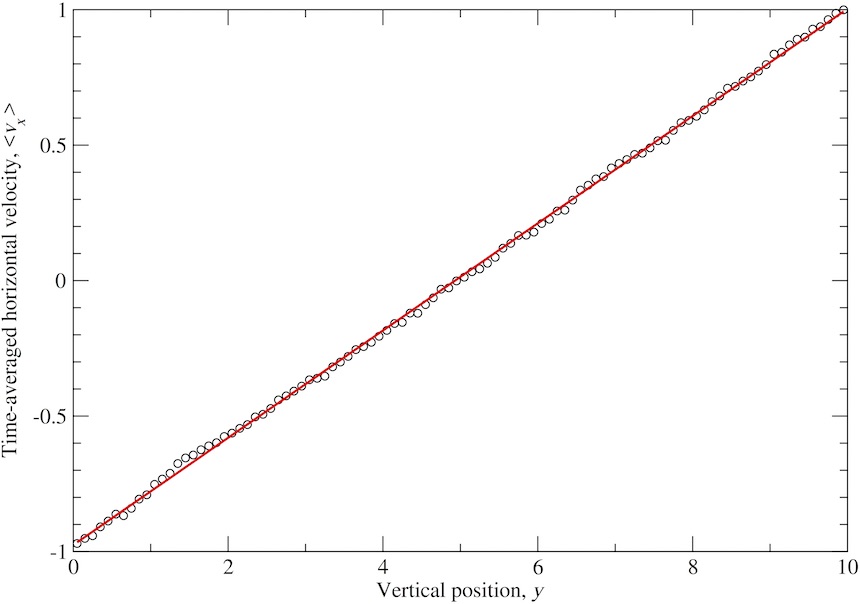
Time-averaged linearly shearing velocity profile obtained from simulation with best-fit line for shear rate determination
VapourLiquid
1000 unbonded water particles are simulated in an elongated box, using many-body (density-dependent) DPD interactions between them to apply both attractions and repulsions [8]. This results in the water particles coalescing into a single body and leaving empty space in the box.
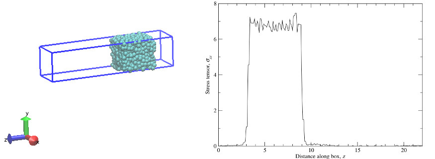
Snapshot of simulation at last time step (left) and time-averaged zz-stress tensor (right)
SurfaceDrop
4000 unbonded water particles are simulated in a box with frozen particle walls at the top and bottom, using many-body DPD interactions between them with stronger repulsions between water and wall particles to represent a hydrophobic surface and a constant body force pointed downwards to represent gravity [9]. This results in coalescing water drops forming on the surface of the bottom wall, with the water-wall repulsion strength dictating the contact angle. (Video)
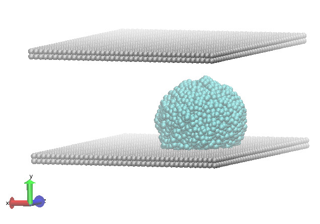
Snapshot of simulation at last time step
References
- Inamuro, T, Yoshino, M, Inoue, H, Mizuno, R and Ogino, F (2002), A lattice Boltzmann method for a binary miscible fluid mixture and its application to a heat-transfer problem, J Comp Phys 179 (1), 201-215
- Halliday, I, Law, R, Care, CM and Hollis, A (2006), Improved simulation of drop dynamics in a shear flow at low Reynolds and capillary number, Phys Rev E 73 (5), 056708
- Yuan, P and Schaefer, L (2006), Equations of state in a lattice Boltzmann model, Phys Fluids 18 (4), 042101
- González-Melchor, M, Mayoral, E, Velázquez, ME and Alejandre, J (2006), Electrostatic interactions in dissipative particle dynamics using the Ewald sums, J Chem Phys 125 (22), 224107
- Jury, S, Bladon, P, Cates, M, Krishna, S, Hagen, M, Ruddock, N and Warren, P (1999), Simulation of amphiphilic mesophases using dissipative particle dynamics, Phys Chem Chem Phys 1 (9), 2051-2056
- Yamamoto, S, Maruyama, Y and Hyodo, S (2002), Dissipative particle dynamics study of spontaneous vesicle formation of amphiphilic molecules, J Chem Phys 116 (13), 5842-5849
- Shillcock, JC and Lipowsky, R (2002), Equilibrium structure and lateral stress distribution of amphiphilic bilayers from dissipative particle dynamics simulations, J Chem Phys 117 (10), 5048-5061
- Ghoufi, A and Malfreyt, P (2011), Mesoscale modelling of the water liquid-vapor interface: A surface tension calculation, Phys Rev E 83 (5), 051601
- Johansson, E (2012), Simulating fluid flow and heat transfer using dissipative particle dynamics, Project report, Department of Energy Sciences, Faculty of Engineering, Lund University, Sweden